
Proxy Modeling of Hydraulic Fractured Wells using Machine Learning and the Subsequant Transfer learning for Estimating of Half Fracture Length
By Uchenna Odi , Aramco Americas, Kola Ayeni , Nouf Alsulaiman , Karri Reddy ,Saudi Aramco, Kathy Ball ,Chevron), Mustafa Basri , Cenk Temizel, Saudi Aramco
Introduction
Transfer learning is a powerful machine and deep learning method that allows knowledge gained by training for one task to be transferred to a similar task. It is widely used in computer vision, natural language, and other unstructured data modeling problems where training a model without prior knowledge can take considerable time and iterations. When utilized, transfer learning can save on training time while providing accuracy that translates to business value.
To understand the uniqueness of transfer learning machine consider Figure 1 which illustrates the working setup of traditional machine learning and transfer learning. In traditional machine learning, two models are constructed to estimate domains A and B separately. However, in transfer learning, knowledge gained from training on domain A is used to model and predict domain B.

Figure 1: Traditional supervised learning vs. transfer learning setup (Ruder, 2017)
As consequence of transferring knowledge from domain A to domain B, more business value is realized when compared to directly spending time and resources to separately train domain A and B separately. This business value of transfer learning is apparent for oil and gas operations where solutions to technical challenges hinge on the amount of capital used to attain the respective solution.
Because of the potential business value in oil and gas, others have applied transfer learning to various types of upstream energy problems. Liu et al. (2020) proposed a joint distribution adaptation based Extreme Gradient boosting transfer learning approach to estimate water adsorption of sublayers in water injection well. For their work, machine learning models were trained on historical injection profile of wells to predict the injection wells of new wells. The authors’ application provided accurate results using transfer learning methodology. The scheme of the proposed workflow is shown in Figure 2 and illustrates a joint distribution adaptation to transfer knowledge obtained from a trained source well block to the target well-block with no injection. The machine learning model was Extreme Gradient Boosting and it was used build a predictive model for water absorption.

Figure 2: Workflow of the proposed method (Liu et al. 2020)
Ma et al. (2020) studied gas adsorption in metal-organic frameworks using transfer learning. Metal-organic frameworks (MOF) are considered one of the most promising materials for gas adsorption due to their nano-porous structures. Ma et al. introduced an inductive transfer learning approach for maximizing the accuracy of machine learning models using a limited number of adsorption gas data. The authors did this by first training a deep neural network (DNN) with a database of 13,506 MOF structures for predicting the adsorption capacity of gases. The trained model knowledge was then transferred to another DNN model (with a small number of data, 100 data). It was found that knowledge learned from the source task significantly increased the prediction accuracy of the other model.
Zini et al. (2020) published a seismic data analysis study for bright spots detection using a deep transfer learning framework. Bright spots are considered strong indicators for hydrocarbon accumulation. Adopted machine learning methods using classification workflow and feature extraction are effectively utilized on 2-D seismic with an 85.4 % F1 score. For this deep learning image classification approach, Zini et al. (2020) implemented data augmentation and inductive transfer-learning methods to overcome the limited data challenge, which is a common issue while performing the training process. As result of their approach, Zini et al. (2020) was successful in detecting bright spots from seismic data using convolutional neural networks (CNN).
Zheng and Wang (2020) investigated applying a deep convolutional neural network for oil spill detection. They used a big data set (including 20,000) from Synthetic Aperture Radars (SARs). The massive data set was trained with a deep convolutional learning network (DCNN) for oil spill detection. The workflow of the proposed DCNN is shown in Figure 3. The data set was carried out using Adaboost Multi-Layer Perceptron (AAMLP) for transfer learning in three possible networks, and the best network was used as the leading network. Since the hyper-parameters and the architectures were adjusted, the network no longer needed transfer learning. The data augmentation process was performed only on the training data.

Figure 3: Flow diagram of the proposed DCNN (Zheng and Wang, 2020)
Transfer learning has been widely used in geophysical studies. Specifically, it is used to interpret the seismic data better and increasing the quality of seismic data. Jreij et al. (2018) used transfer learning in a convolutional neural network to quantitatively analyze the added value of surface distributed acoustic sensors in sparse geo-phone arrays. Hu et al. (2019) performed a progressive deep transfer learning study to cycle-skipping full-waveform inversion. They reconstructed the absent low-frequency data by deep learning networks involving dual data feed and progressive transfer learning. A nonlinear relationship between different bands was created. One of the most important outcomes of their study is that the model did not require any prior information of the subsurface geological data.
Xing et al. (2018) studied transfer learning applications on synthetic data to improve faults continuity. Faults are defined as planar fracture shape discontinuities created as the result of tectonic movement in a volume of rock. Manual fault interpretation required too much time and effort. It is more efficient to use automatic fault interpretation, which involved calculating edge attributes and fault likelihoods and extraction of fault surfaces. Xing et al. (2018) proposed a transfer learning method that uses synthetic circle data. The circle data had different connectivity balancing on curvatures and dips. The proposed method was also applied to fault likelihood data with discontinuity. Synthetic data was trained with convolutional and fully connected layers, and the trained models were then used to track faults for testing. Promising results were obtained from the tests performed on synthetic circular datasets and on real fault datasets. As shown in Figure 4, the input discontinuity is improved using the transfer learning method with different techniques. The black ellipsoids show the connected discontinuities. The study concluded that using transfer learning from synthetic circle datasets can significantly improve fault detection.

Figure 4: Test results on fault tracking using Hca dataset (Xing et al. 2018)
In this work, transfer learning is applied to shale gas production for two tasks. The first task was history matching half fracture length across an area of interest. The second task was predicting gas production. To understand the two applications of transfer learning introduced in this work, the generalized methodology and procedure of both proposed applications is discussed.
Methodology
In the context of shale gas reservoirs, transfer learning is utilized by training a machine or deep learning model on existing shale data for a specific task with specific characteristics and applying it to an area of similar characteristics for a similar task. Pan and Yang (2009) explained mathematically the general concept of transfer learning. These authors mathematically conceptualized transfer learning by considering a domain consisting of a feature space and corresponding marginal probability distribution expressed as the following expression.

A title
Image Box text
Where D, corresponds to the domain consisting of a feature space, χ, and marginal distribution, P(X). X is series of data points paired to target points Y in the target output space, γ, expressed as the following.

A title
Image Box text
Pan and Yang then defined a machine or deep learning tasks in the same language as the domain space in the following expression.

A title
Image Box text
Where T represents the task domain consisting of a target output space, γ, and the function, η, which predicts yi as a function xi. Transfer learning can then be defined as learning the target conditional probability distribution, P(YT|XT), in the target domain, DT, by using the information trained from source tasks, Ts, in the domain, DS.
Applying the generalized transfer learning methodology to half fracture length and gas production rate requires creating a predictive model that trains from a known domain consisting of shale gas data, and then transferring the conditional probability generated by the machine learning tasks onto the target domain. The application and procedure for transfer learning for half fracture length is discussed which uses several novel components.
Transfer Learning for Half Fracture Length Prediction
Inferring half fracture after a hydraulic fracturing task can be difficult and generally requires several history matching iterations in a finite difference simulator. In this work, transfer learning is used in conjunction with hydraulic fracturing simulation and probabilistic sampling. Specifically, the procedure for applying the transfer learning methodology to half fracture length prediction involved utilizing a hydraulic fracturing simulator, Monte Carlo Sampling, and machine learning. The steps of this process are outlined as the following:
- Generate sensitivities using Monte Carlo sampling related to hydraulic fracturing in shale reservoirs.
- Run each hydraulic fracturing sensitivity in a hydraulic fracturing simulator and store as a central data set used for machine learning training. This data set serves as the source domain for transfer learning.
- Create machine learning model of half fracture length using the generated hydraulic fracturing sensitivities as inputs and the corresponding half fracture length as a target parameter. This generalized step serves as the source task.
- Appy machine learning half fracture length prediction across target domain.
For the first step, generating sensitivities of hydraulic fracturing, parameters ranges were defined for subsequent probabilistic sampling. Table 1 corresponds to the parameter ranges sampled that described a hydraulic fracturing process in a wet gas to dry gas reservoir.

Table 1: Hydraulic Fracturing Sensitivity Parameter Ranges
Using the parameter ranges, 2,000 realizations of hydraulic fracturing were randomly generated using Monte Carlo sampling. For the second step of the proposed process, these realizations were simulated in a hydraulic fracturing simulator which models a hydraulically fractured well where the interference between each fracture is accounted for using spatial superposition theory.

(a)

(b)
Figure 5: Generalized Hydraulic Fracture Simulator Schematic and Assumptions (a) Hydraulic Fracture Single Well System (b) Interference Between Each Fracture.
Using superpositioning theory, the interference between each fracture was modeled and accounted for in a matrix expression which incorporates respective pressure drops and rates from the fracture well system. For example, a four fracture system results in a four by four matrix represented in the following expression.

A title
Image Box text
Where pD corresponds to the dimensionless pressure drop from a fracture and qD corresponds to the dimensionless rate from a fracture. For instance, the interference between the first and second fracture corresponds to pD12 and the rate from the first fracture corresponds to qD1. The analytical solution for dimensionless pressure can then expressed as the following equation.

A title
Image Box text
Where SxD is the source function aligned to the x axis, SyD is the source function aligned to the y axis. Further details about the hydraulic fracture analytical solution formulation can be found in Horne and Temeng’s publication (Horne and Temeng, 1995).
As a result of running each realization of hydraulic fracturing, the corresponding statistical attributes of all generated sensitivities and corresponding gas production rate are displayed in Table 2.

Table 2: Statistical Ranges for Hydraulic Fracturing Monte Carlo Sampling and Simulation
Having now defined the source domain (represented by the generated hydraulic fracturing sensitivities) and the source target (half fracture length generated from sensitivities), a machine learning task was designed to estimate half fracture length as a function of the hydraulic fracturing parameters. In this third step of the overall workflow, the machine learning task was created by using the hydraulic fracturing sensitivities to train a gradient boost machine learning model. The resulting prediction accuracy of the machine learning prediction for half fracture is outlined in Figure 6.

Figure 6: Cross Validation Results for Half Fracture Length Machine Learning Prediction from Monte Carlo Sampling
Figure 6 illustrates that the gradient boost model approximately models the half fracture length generated from Monte Carlo sensitivity simulation. The resulting machine learning model had a root mean square error of the validation, cross validation, and holdout set of 3.69 feet, 3.72 feet, and 3.87 feet respectively. The relative importance (Figure 7) of the parameters was calculated and revealed a ranking of essentiality for each feature used to predict half fracture length from simulation data.

Figure 7: Relative Feature of Importance for Half Fracture Length Machine Learning Prediction from Monte Carlo Sampling
The relative feature of importance reveals an approximate understanding of the parameters that contribute significantly to the half fracture length prediction.
To test the effectiveness of the trained machine learning model, transfer learning methodology was utilized to deploy the machine learning model across the Eagle Ford shale data set. The Eagle Ford data set served as a target domain and it comprised of more than 20,000 wells with statistical characteristics summarized in Table 3.

Table 3: Statistical Summary of the Eagle Ford
Using transfer learning, the machine learning prediction for half fracture length was applied to the Eagle Ford data in the fourth step of the overall process. Mapped out results (Figure 8) reveal the generalized half fracture length prediction across the Eagle Ford basin.

Figure 8: Eagle Ford Average Half Fracture Length
With estimates of half fracture length across the Eagle Ford shale data set, an approximate understanding of the half fracture length was created. The Eagle Ford shale data, including the half fracture length estimate, was then combined with the hydraulic fracturing data set generated by Monte Carlo sampling. A history matched model for gas production using the transfer learning half fracture length prediction was then generated by creating a machine learning gas production prediction using the combined data set as the domain source. A decision tree machine learning algorithm was utilized for the task of predicting gas production as function of the combined Eagle Ford and Monte Carlo sensitivity generated data set properties. The corresponding root mean square error of the gas production decision tree machine learning prediction was 340 MSCF/Day, 338 MSCF/Day, and 354 MSCF/Day for the validation, cross validation and holdout set. A summary of model results (Figure 9) show the effectiveness of history matching half fracture length using the transfer learning methodology.

(a)

(b)
Figure 9: Eagle Ford History Matched Results (a) Average Gas Production (b) Cumulative Gas Production
The average gas production across the Eagle Ford data set approximately matches the average predicted gas production through normalized time. In addition, the predicted cumulative volume similarly matches the Eagle Ford cumulative volume data. Results illustrate the overall success of history matching half fracture length using transfer learning methodology. Further results from LaSalle and Frio County (Figure 10 and Figure 11) illustrate how powerful the transfer learning methodology is in approximating half fracture length and correspondingly predicting gas production and cumulative production for respective counties in the Eagle Ford.

(a)

(b)
Figure 10: History Matched Average Gas Production for Eagle Ford Areas (a) Frio County (b) La Salle County

Figure 11: History Matched Cumulative Gas Production for Eagle Ford Counties
Transfer Learning for Gas Production Rate Prediction
In the previous section transfer learning was successfully implemented to predict half fracture length and to subsequently history match Eagle Ford gas production. In many cases, predicting gas production in un-drilled locations is a challenge in addition to estimating half fracture length. To solve this problem a transfer learning methodology was utilized. To illustrate the transfer learning approach, the transfer learning methodology was applied to the Eagle Ford shale data set where La Salle County was used as a training set to predict gas production from Frio, McMullen, Webb, and Dimmit county. In this application, La Salle county data served as the source domain data set while Frio, McMullen, Webb, and Dimmit County served as the target domains. La Salle was chosen because of its representative fluid windows (Figure 12) observed in Frio, McMullen, Webb, and Dimmit counties.
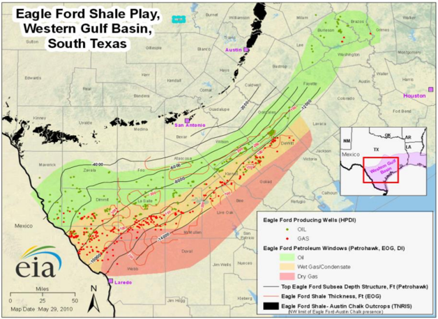
Figure 12: Eagle Ford Fluid Window (EIA, 2014)
The generalized methodology of applying transfer learning for the purpose of shale gas forecasting involved the following steps:
- Collect reservoir, completion, geological, and engineering parameters across wells with gas production history. Apply transfer learning half fracture length model on wells with production history.
- Using area of interest data, train machine learning model using half fracture length as target parameter.
- Train machine learning and deep learning model for gas production prediction using area with gas production history.
- Collect reservoir, completion, geological, and engineering parameters across potential well locations with unknown gas production history.
- Use machine learning model of half fracture length trained on area with known production history to make prediction of half fracture length of area with unknown production history.
- Apply transfer learning gas production model onto area with unknown history for gas production prediction and forecasting.
For the first step, well level data was collected across La Salle County and the transfer learning half fracture length model was deployed using the well level production history. A summary of La Salle’s data including the half fracture length is displayed in Table 4.

Table 4: Statistical Summary of the La Salle County
To determine the half fracture length of an area with no prior production history, required building a new machine learning model that did not include gas production rate as one of the inputs. A random forest machine learning model was chosen, and the resulting machine learning model had a root mean square error validation, cross validation, and holdout of 2.84 feet, 2.85 feet, and 2.79 feet respectively. The relative importance of the parameters was calculated and revealed a ranking of essentiality of each feature used to predict half fracture length from La Salle county field data (Figure 13). The relative importance for permeability, tubing diameter, number of fractures, and bottomhole pressure were found to be not important due to the small standard deviation of each parameter revealed in Table 4. Furthermore, number of fractures and bottom hole pressure were approximate assumptions for the area and thus spatial variability was purposely omitted for these parameters in this work. Finally, mapped out results (Figure 14) illustrate the generalized geospatial distribution of the half fracture length prediction across La Salle county.

Figure 13: Relative Feature of Importance for Half Fracture Length Random Forest Machine Learning Prediction from La Salle County Data

Figure 14: Geospatial Distribution of La Salle County Half Fracture Length Prediction
The next step in the workflow required using transfer learning methodology to train a machine and deep learning model for gas prediction. To do this, a gradient boost machine learning model and a deep learning neural network (ANN) was constructed for comparison. The gradient boost machine learning model had a root mean square error of 234 MSCF/Day, 250 MSCF/Day, and 229 MSCF/Day for the validation, cross validation, and holdout set respectively. The deep learning model contained eight hidden layers. The number of nodes in each layer listed in order were 1024, 512, 256, 128, 64, 32, 16, and 8 units. The deep learning model had a root mean square error of 245 MSCF/Day, 254 MSCF/Day, and 248 MSCF/Day for the validation, cross validation, and holdout set respectively. Comparing the gradient boost and deep learning model cross validation results (Figure 15), it is apparent that the models approximately estimate La Salle county’s gas production rate.

Figure 15: Cross Validation Results for Gas Production Machine Learning Prediction from La Salle County Data
Feature importance comparisons, shown in Figure 16, illustrate the primary differences and similarities between the gradient boost and the deep learning model. Together, both models indicate that tubing diameter, number of fractures, and bottom hole pressure were not essential to predicting gas production. This was because there was not enough variability in these parameters as indicated in Table 4. These parameters were assumed to be a constant parameter for machine learning purposes. Looking at the other parameters, both models indicate that varied ranking of importance with time being the most important parameter. Both models can be compared to fitting production decline data using a decline curve equation as a function of time and other hyper parameters. The primary difference with using machine learning and gradient boost is that additional parameters beyond hyper parameters directly influence the performance of the respective models and thus provide more robustness in predicting a decline when compared to traditional decline curve methods.

(a)

(b)
Figure 16: Relative Feature of Importance (a) Gradient Boost (b) ANN
Deploying the prediction across all La Salle’s data, Figure 17 shows the effectiveness of both models in predicting average gas production through normalized time. Deploying both transfer learning models to Dimmit, Frio, McMullen, and Webb county demonstrates the effectiveness in predicting the cumulative production (Figure 18) using machine learning and deep learning.

Figure 17: La Salle Average Gas Production Comparison

Figure 18: Cumulative Gas Production Prediction for Eagle Ford Counties Using Transfer Learning
Conclusions
Transfer learning was applied to Eagle Ford production in two primary ways which are half fracture length prediction and gas production prediction. Both applications reveal the usefulness in using transfer learning to predict gas production and cumulative volume approximately.
Using transfer learning for half fracture length provided an avenue to history match gas production using machine learning. For that application, transfer learning was demonstrated by transferring the machine learning gained from training the probabilistic hydraulic fracturing simulations and applying it to the Eagle Ford production history for history matching.
Applying transfer learning for gas production prediction provided a method to estimate gas production in un-drilled locations. For that application, transfer learning was demonstrated by transferring the machine learning and deep learning gained from training La Salle County’s shale data and applying it to specific nearby counties for estimating cumulative gas volume.